2. User Guide

Spectrum provides classes and functions to estimate Power Spectral Densities (PSD hereafter). This documentation will not describe PSD theoritical background, which can be found in many good books and references. Therefore, we consider that the reader is aware of some terminology used here below.

2.1. QuickStart (Periodogram example)

Spectrum can be invoked from a python shell. No GUI interface is provided yet. We recommend to use ipython, which should be started with the pylab option:

ipython --pylab

Then, the simplest way to start with Spectrum is to import everything from the library:

from spectrum import *

In the following examples, we will use data_cosine() to generate a toy data sets:

data = data_cosine(N=1024, A=0.1, sampling=1024, freq=200)

where data contains a cosine signal with a frequency of 200Hz buried in white noise (amplitude 0.1). The data has a length of N=1024 and the sampling is 1024Hz.

We can analyse this data using one of the Power Spectrum Estimation method provided in spectrum. All methods can be found as functions or classes. Although we strongly recommend to use the object oriented approach, the functional approach may also be useful. For now, we will use the object approach because it provides more robustness and additional tools as compared to the functional approach (e.g., plotting). So, let us create a simple periodogram:

p = Periodogram(data, sampling=1024)

Here, we have created an object Periodogram. No computation has been performed yet. To run the actual estimation, you can use either:

p() # now you run the estimation

or:

p.run()

and finally, you can plot the resulting PSD:

p.plot(marker='o')  # standard matplotlib options are accepted

[hires.png, pdf]

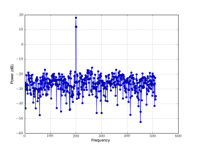
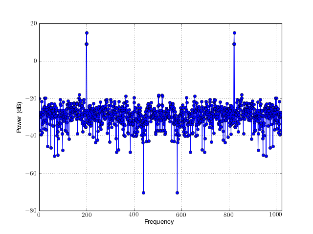
Since the data is purely real, the PSD (stored in p.psd) is a onesided PSD, with positive frequencies only. If the data were complex, the two-sided PSD would have been computed and plotted. For the real case, you can still plot a two-sided PSD by setting the sides option manually:

p.plot(sides='twosided')

[hires.png, pdf]

You can also look at a centered PSD around the zero frequency:

p.plot(sides='centerdc')

Warning

By convention, the psd attribute contains the default PSD (either one-sided for real data or two-sided for the complex data).

Since p is an instance of Periodogram, you can introspect the object to obtain diverse information such as the original data, the sampling, the PSD itself and so on:

p.psd # contains the PSD values
p.frequencies() returns a list of frequencies
print(p) # prints some information about the PSD.

2.2. The object approach versus functional approach (ARMA example)

2.2.1. Object approach

In the previous section, we’ve already illustrated the object approach using a Fourier-based method with the simple periodogram method. In addition to the Fourier-based PSD estimates, Spectrum also provides parametric-based estimates. Let us use parma() class as a second illustrative example of the object approach:

from spectrum import parma

Many functionalities available in Spectrum are inspired by methods found in [Marple]. The data sample used in most of the examples is also taken from this reference and can be imported as follows (this is a 64 complex data samples):

from spectrum import marple_data

The class parma allows to create an ARMA model and to plot the PSD, similarly to the previous example (Periodogram). First, we need to create the object:

p = parma(marple_data, 15, 15, 30, NFFT=4096)

where 15,15 and 30 are arguments of the ARMA model (see spectrum.parma), and NFFT is the number of final points.

Then, computation and plot can be performed:

p.run()
p.plot(norm=True, color='red', linewidth=2)

[hires.png, pdf]

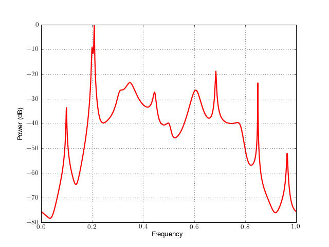
Since the data is complex, the PSD (stored in p.psd) is a twosided PSD. Note also that all optional arguments accepted by matplotlib function are also available in this implementation.

2.2.2. Functional approach

The object-oriented approach can be replaced by a functional one if required. Nevertheless, as mentionned earlier, this approach required more expertise and could easily lead to errors. The following example is identical to the previous piece of code.

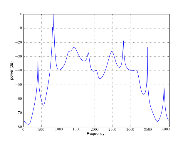
In order to extract the autoregressive coefficients (AR) and Moving average coefficients (MA), the arma_estimate() can be used:

from spectrum.arma import arma_estimate, arma2psd
ar, ma, rho = arma_estimate(marple_data, 15, 15, 30)

Once the AR and/or MA parameters are found, the arma2psd() function creates a two-sided PSD for you and the PSD can be plotted ad follows:

from spectrum import arma_estimate, arma2psd, marple_data
from pylab import *
ar, ma, rho = arma_estimate(marple_data, 15, 15, 30)
psd = arma2psd(ar, ma, rho=rho, NFFT=4096)
plot(10*log10(psd/max(psd)))
axis([0, 4096, -80, 0])
xlabel('Frequency')
ylabel('power (dB)')
grid(True)

[hires.png, pdf]

Note

1. The parameter 30 (line 3) is the correlation lag that should be twice as much as the required AR and MA coefficient number (see reference guide for details).
2. Then, we plot the PSD manually (line 5), and normalise it so as to use dB units (10*log10)
3. Since the data are complex data, the default plot is a two-sided PSD.
4. The frequency vector is not provided.