5.2. Multitapering¶

Multitapering method.

This module provides a multi-tapering method for spectral estimation. The computation of the tapering windows being computationally expensive, a C module is used to compute the tapering window (see spectrum.mtm.dpss()).

The estimation itself can be performed with the spectrum.mtm.pmtm() function

dpss(N, NW=None, k=None)¶

Discrete prolate spheroidal (Slepian) sequences

Calculation of the Discrete Prolate Spheroidal Sequences also known as the slepian sequences, and the corresponding eigenvalues.

Parameters:

Parameters:	N (int) – desired window length NW (float) – The time half bandwidth parameter (typical values are 2.5,3,3.5,4). k (int) – returns the first k Slepian sequences. If k is not provided, k is set to NW2*.
Returns:	tapers, a matrix of tapering windows. Matrix is a N by k (k is the number of windows) eigen, a vector of eigenvalues of length k

N (int) – desired window length
NW (float) – The time half bandwidth parameter (typical values are 2.5,3,3.5,4).
k (int) – returns the first k Slepian sequences. If k is not provided, k is set to NW*2.

Returns:

tapers, a matrix of tapering windows. Matrix is a N by k (k is the number of windows)
eigen, a vector of eigenvalues of length k

The discrete prolate spheroidal or Slepian sequences derive from the following time-frequency concentration problem. For all finite-energy sequences index limited to some set , which sequence maximizes the following ratio:

$\lambda = \frac{\int_{-W}^{W}\left| X(f) \right|^2 df} {\int_{-F_s/2}^{F_s/2}\left| X(f) \right|^2 df}$

where $F_s$ is the sampling frequency and $|W| < F_s/2$ . This ratio determines which index-limited sequence has the largest proportion of its energy in the band $[-W,W]$ with $0 < \lambda < 1$ . The sequence maximizing the ratio is the first discrete prolate spheroidal or Slepian sequence. The second Slepian sequence maximizes the ratio and is orthogonal to the first Slepian sequence. The third Slepian sequence maximizes the ratio of integrals and is orthogonal to both the first and second Slepian sequences and so on.

Note

Note about the implementation. Since the slepian generation is computationally expensive, we use a C implementation based on the C code written by Lees as published in:

Lees, J. M. and J. Park (1995): Multiple-taper spectral analysis: A stand-alone C-subroutine: Computers & Geology: 21, 199-236.

However, the original C code has been trimmed. Indeed, we only require the multitap function (that depends on jtridib, jtinvit functions only).

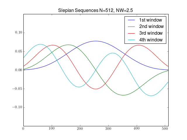
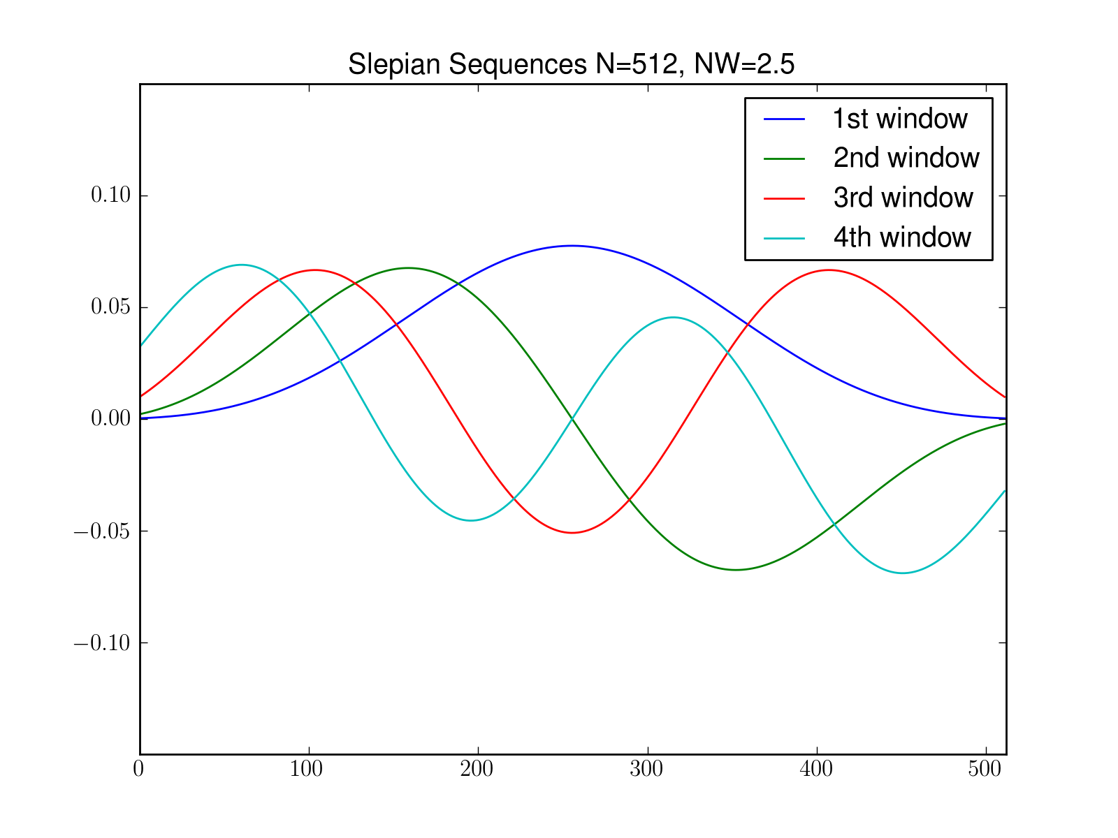
from spectrum import *
from pylab import *
N = 512
[w, eigens] = dpss(N, 2.5, 4)
plot(w)
title('Slepian Sequences N=%s, NW=2.5' % N)
axis([0, N, -0.15, 0.15])
legend(['1st window','2nd window','3rd window','4th window'])

[hires.png, pdf]

Windows are normalised:

$\sum_k h_k h_k = 1$

References :

References :	[Percival] Slepian, D. Prolate spheroidal wave functions, Fourier analysis, and uncertainty V: The discrete case. Bell System Technical Journal, Volume 57 (1978), 1371430

[Percival]

Slepian, D. Prolate spheroidal wave functions, Fourier analysis, and uncertainty V: The discrete case. Bell System Technical Journal, Volume 57 (1978), 1371430

Note

the C code to create the slepian windows is extracted from original C code from Lees and Park (1995) and uses the conventions of Percival and Walden (1993). Functions that are not used here were removed.

pmtm(x, NW=None, k=None, NFFT=None, e=None, v=None, method='adapt', show=True)¶

Multitapering spectral estimation

Parameters:	x (array) – the data NW (float) – The time half bandwidth parameter (typical values are 2.5,3,3.5,4). Must be provided otherwise the tapering windows and eigen values (outputs of dpss) must be provided k (int) – uses the first k Slepian sequences. If k is not provided, k is set to NW2*.

:param NW :param e: the matrix containing the tapering windows :param v: the window concentrations (eigenvalues) :param str method: set how the eigenvalues are used. Must be in [‘unity’, ‘adapt’, ‘eigen’] :param bool show: plot results

Usually in spectral estimation the mean to reduce bias is to use tapering window. In order to reduce variance we need to average different spectrum. The problem is that we have only one set of data. Thus we need to decompose a set into several segments. Such method are well-known: simple daniell’s periodogram, Welch’s method and so on. The drawback of such methods is a loss of resolution since the segments used to compute the spectrum are smaller than the data set. The interest of multitapering method is to keep a good resolution while reducing bias and variance.

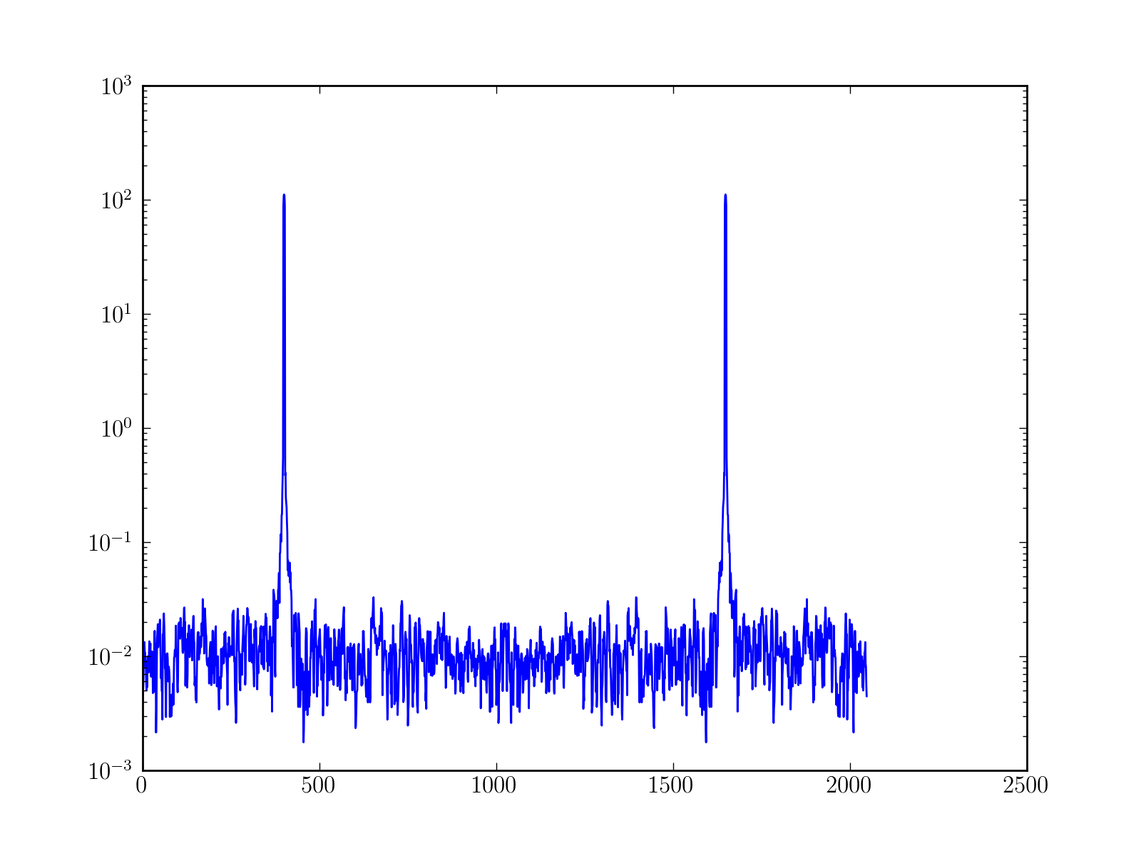
How does it work? First we compute different simple periodogram with the whole data set (to keep good resolution) but each periodgram is computed with a different tapering windows. Then, we average all these spectrum. To avoid redundancy and bias due to the tapers mtm use special tapers.

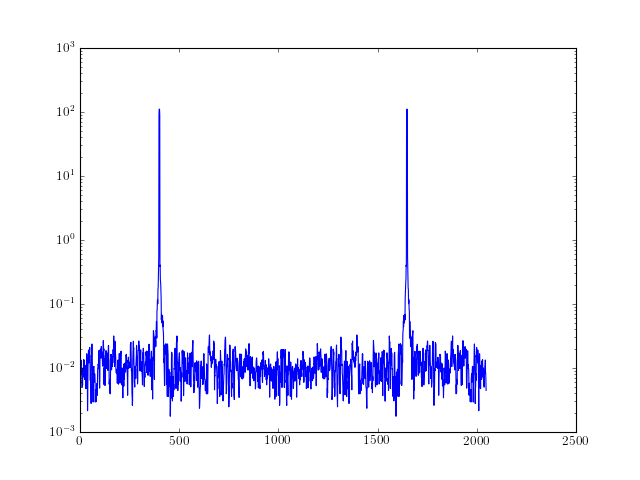
from spectrum import *

data = data_cosine(N=2048, A=0.1, sampling=1024, freq=200)
# If you already have the DPSS windows
[tapers, eigen] = dpss(2048, 2.5, 4)
res = pmtm(data, e=tapers, v=eigen, show=False)
# You do not need to compute the DPSS before end
res = pmtm(data, NW=2.5, show=False)
res = pmtm(data, NW=2.5, k=4, show=True)

[hires.png, pdf]

Front page|Spectrum - Spectral Analysis in Python (0.5.2)

5.2. Multitapering¶

Search

Table Of Contents